Introduction
The van der Waals equation of state was presented by Johannes Diderik van der Waals in his 1873 PhD thesis1, which describes the state of matter under a given set of physical conditions, such as pressure, volume, temperature, or internal energy. At the time of writing his thesis, the existence of molecules was not accepted, rather opposed. However, he was convinced that molecules existed.
Later in 1910, van der Waals was awarded the Nobel Prize in Physics for his contributions2. An excerpt from his is Nobel Lecture says,
“It will be perfectly clear that in all my studies I was quite convinced of the real existence of molecules, that I never regarded them as a figment of my imagination, nor even as mere centres of force effects. I considered them to be the actual bodies, thus what we term “body” in daily speech ought better to be called “pseudo body”. It is an aggregate of bodies and empty space. We do not know the nature of a molecule consisting of a single chemical atom. It would be premature to seek to answer this question but to admit this ignorance in no way impairs the belief in its real existence… When I began my studies, I had the feeling that I was almost alone in holding that view… Many of those who opposed it most have ultimately been won over, and my theory may have been a contributory factor.”
This article demonstrates how to program van der Waals equation of state in python and produce 2D and 3D visualisations of PVT diagram. The explanation of different terms in the van der Waals equation of state, their interpretations and significance are available out there for interested readers 3,4.
Equations
The mathematical formulation of van der Waals equation of state may be written as:
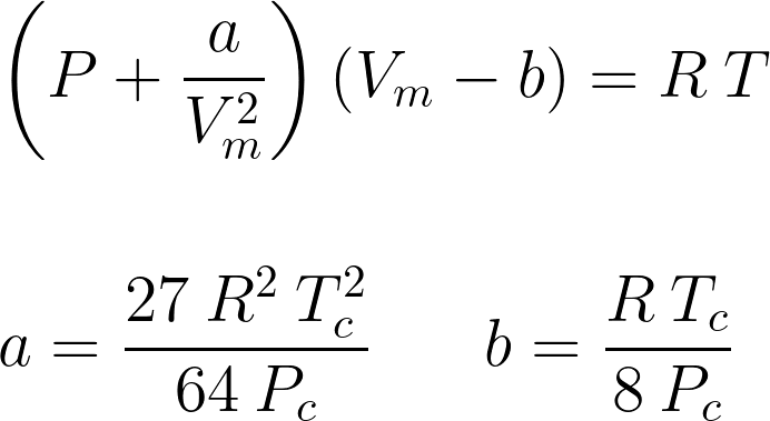
Where, P is pressure, a and b are substance-specific constants which can be calculated by critical temperature (Tc), critical pressure (Pc) and universal gas constant (R), Vm is molar volume, T is temperature.
Python Implementation
Let’s start with importing necessary packages to compute and produce 2D as well as 3D visualisations of PVT curve.
import numpy as np
import matplotlib as mpl
import matplotlib.pyplot as plt
import plotly as py
import plotly.graph_objects as go
Next, for demonstration I chose CO2 as a substance and its critical parameters are defined as shows below,
######## CO2 data ########

Tc = 304            # Critical temperature, K
Pc = 73.6           # Pressure, Bar
Pc = Pc*100000      # Converting pressure units, Pa
R = 8.314           # Universal gas constant, (m3.Pa)/(mol.K)
In the following steps, a temperature and molar volume ranges are chosen and discretised for which pressures will be computed.
######## Temperature Range ########

T1, T2 = -50, 120                         # Start and end temperatures, °C
T_step = 10                               # Step size, °C
T = np.arange(T1+273.15,T2+273.15,T_step) # Discretisation and temperature conversion

######## Molar Volume Range ########

V1, V2 = 0.00006, 0.001     # Start and end molar volume, m3
V_step = 0.000001           # Step size, m3
V = np.arange(V1,V2,V_step) # Discretisation
The below function computes, substance-specific constants (a, b) and pressure at each discretized value of temperature and pressure.
######## Pressure Calculation ########

def vdw(T,V):

    # Substance-specific constants
    a = (27*R**2*Tc**2)/(64*Pc)
    b = (R*Tc)/(8*Pc)

    P = np.zeros((len(T),len(V)))
    for i in range(0,len(T)):
        for j in range(0,len(V)):
            P[i,j] = ((R*T[i])/(V[j]-b) - a/V[j]**2)/100000
            # print(P)
    return P

P_vdw = vdw(T,V)
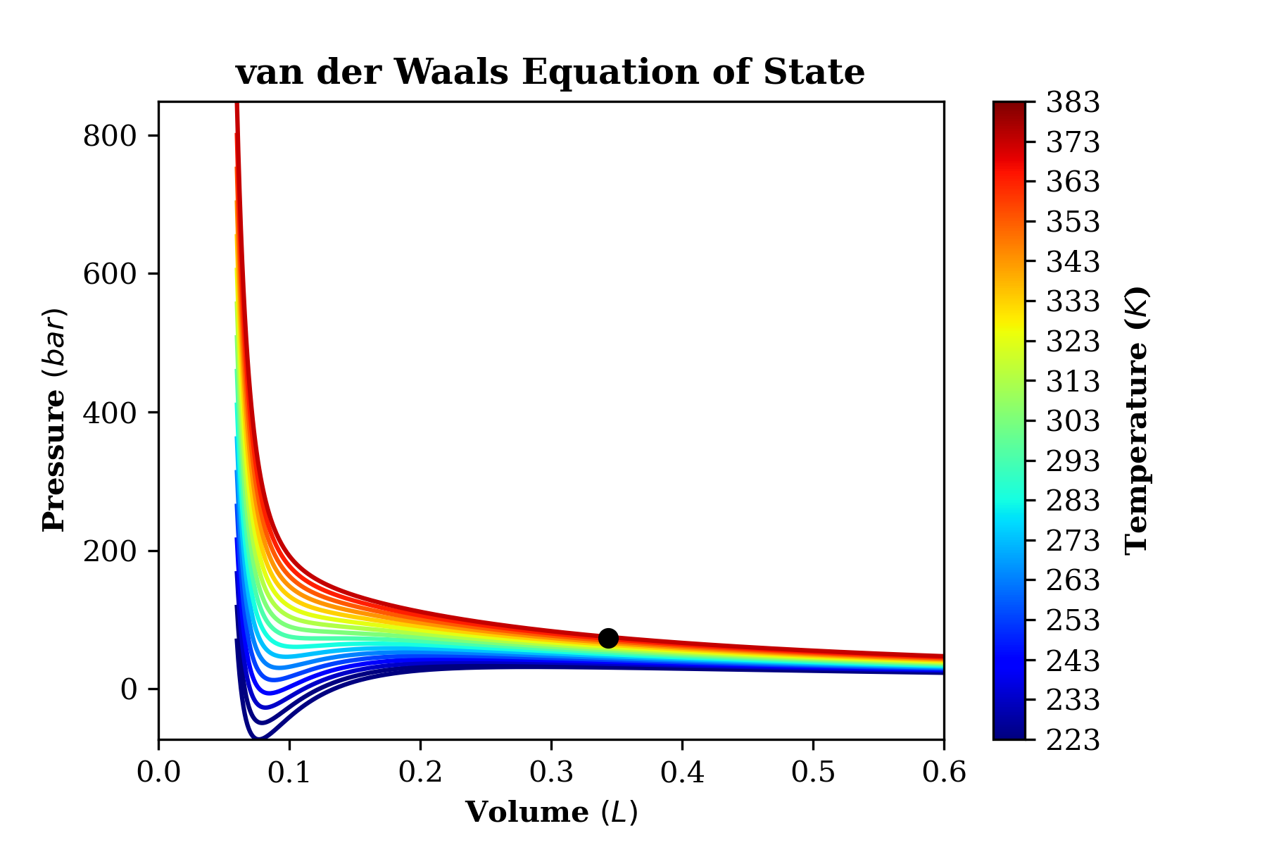
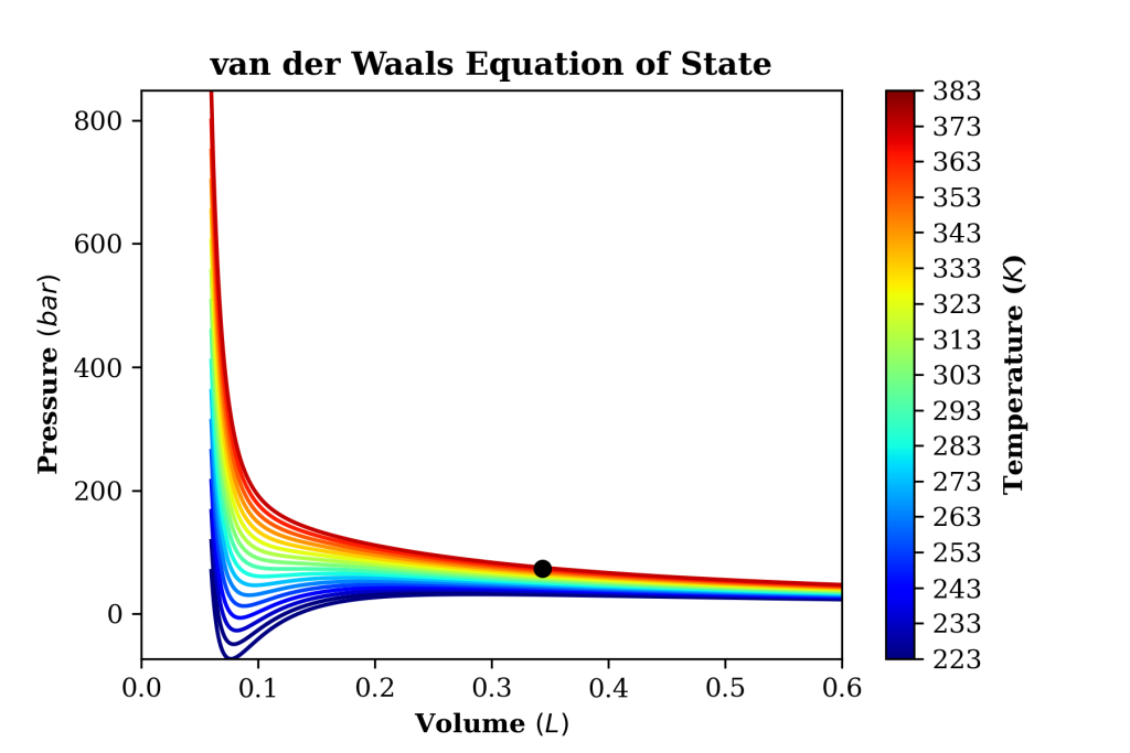
2D Visualisation
The below lines of code will produce a 2D visualisation of the PVT diagram and will save the image in PNG format. Note that for “nicer” visualisation, molar volume units are converted from m3 to L.
######## 2D Visualisation ########

plt.figure(num=1, dpi=300)
plt.rcParams["font.family"] = "serif"
plt.rcParams['figure.facecolor'] = 'white'

c = np.arange(1, len(T) + 1 )
norm = mpl.colors.Normalize(vmin=c.min(), vmax=c.max())
cmap = mpl.cm.ScalarMappable(norm=norm, cmap=mpl.cm.jet)
cmap.set_array([])

for i, yi in enumerate(P_vdw):
    plt.plot(V*1000, yi, c = cmap.to_rgba(i))

plt.plot([0 , 0.001], [0, 0], 'k--') # zero line
plt.plot((R*Tc)/Pc*1000,Pc/100000,'ko',markersize=6) # Critical point
plt.xlim([0, 0.6])
plt.ylim([P_vdw.min(),P_vdw.max()])

cbar=plt.colorbar(cmap, ticks=c)
# cbar.set_ticks(c)
cbar.set_ticklabels(T)
cbar.ax.set_yticklabels(["{:.0f}".format(i)+" " for i in T])
cbar.ax.set_ylabel('Temperature ($K$)', weight="bold")

plt.title("van der Waals Equation of State", weight="bold")
plt.xlabel("Volume $(L)$", weight="bold")
plt.ylabel("Pressure $(bar)$", weight="bold")
plt.savefig('vdw.png')
plt.show()
Output:
3D Visualisation
The below lines of code will produce a 3D visualisation of the PVT diagram and will save the image in html format. Note that for “nicer” visualisation, molar volume units are converted from m3 to L.
######## 3D Visualisation ########

X, Y = np.meshgrid(V*1000, T)
Z = P_vdw

fig = go.Figure(data=[go.Surface(z=Z, x=Y, y=X, colorscale ='Viridis')])

fig.update_layout(title='Van der Waals Equation of State',
                  font=dict(color="Black"),
                  width=800, height=600,
                  margin=dict(l=65, r=50, b=50, t=50),
                  scene =
                          dict(yaxis = dict(nticks=10, range=[0, 0.6],),
                               xaxis = dict(nticks=T_step, range=[T.max(), T.min()+T_step],),
                               zaxis = dict(nticks=10, range=[P_vdw.min(),P_vdw.max()],),

                               yaxis_title="Volume (L)",
                               xaxis_title='Temperature (K)',
                               zaxis_title='Pressure (bar)'
                              )
                  )

fig.update_layout(hovermode="x")
fig.update_traces(showscale=False)
fig.write_html(r"YOUR_PATH\file.html")
py.offline.plot(fig, filename="vdw.html")
fig.show()
Output:
Last Remarks
This concludes the implementation of van der Waals equation of state in python. This article is written only for educational purposes and to express my love for programming 😉. Lastly, I am not a professional programmer so (I know that) this code is far from optimum but most importantly it works! 😊 Any constructive feedback is welcome.
Sources
- Over de Continuited van den Gas-en Vloeistoftoestand, van der Waals, J.D. (1873)
- Nobel Lecture
- Introduction to Chemical Engineering Thermodynamics, J.M. Smith, Hendrick C Van Ness, Michael Abbott (2005)
- Taking Another Look at the van der Waals Equation of State–Almost 150 Years Later, Kontogeorgis (2019)
2 Comments
Pushkar · February 16, 2022 at 5:47 pm
3D visualization is cool.
Modified Redlich-Kwong-Soave Equation of State – Pushkar S. Marathe · April 30, 2022 at 1:00 pm
[…] In my previous article, I demonstrated the implementation of Van der Waals equation of state in Python. In this article, […]