Introduction
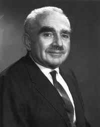
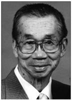
In 1949 [1] , Otto Redlich and Joseph Neng Shun Kwong introduced their version of equation of state which was considered to be a notable improvement to the van der Waals equation. Later in 1972 [2], Giorgio Soave modified it by assuming that the parameter a in the original equation to be temperature-dependent.


In my previous article, I demonstrated the implementation of Van der Waals equation of state in Python. In this article, let us look at the pythonic implementation of Modified of Redlich-Kwong-Soave Equation of State.
Equations
The mathematical formulation of modified Redlick-Kwong-Soave may be written as [3]:

Where, P is pressure, a and b are substance-specific constants which can be calculated by critical temperature (Tc), critical pressure (Pc) and universal gas constant (R), Vm is molar volume, T is temperature, and α called as the attractive term accounts the influence of acentric factor (ω) and temperature.
Python Implementation
Let’s start with importing necessary packages to compute and produce 2D visualisation of PVT curve.
import numpy as np
import matplotlib.pyplot as plt
Next, for demonstration I chose CO2 as a substance, and its critical parameters and acentric factor are defined as shows below,
# CO2 data
Tc = 304 # K
Pc = 73.6 # Bar
Pc = Pc*100000 # Pa
R = 8.314 # (m3.Pa)/(mol.K)
omega = 0.228
In the following steps, a temperature and molar volume ranges are chosen and discretised for which pressures will be computed.
######## Temperature Range ########

T1, T2 = -50, 120                         # Start and end temperatures, °C
T_step = 10                               # Step size, °C
T = np.arange(T1+273.15,T2+273.15,T_step) # Discretisation and temperature conversion

######## Molar Volume Range ########

V1, V2 = 0.0000425, 0.001     # Start and end molar volume, m3
V_step = 0.000001           # Step size, m3
V = np.arange(V1,V2,V_step) # Discretisation
The below function computes, substance-specific constants (a, b), attractive term (α) and pressure at each discretized value of temperature and pressure.
##### Pressure Calculation #####

def RKS(T,V):

    # Constants
    a = (0.42747*R**2*Tc**2)/(Pc)
    b = (0.08664*R*Tc)/(Pc)

    P = np.zeros((len(T),len(V)))
    for i in range(0,len(T)):
        for j in range(0,len(V)):
            alpha = (1 + (0.48508 + 1.55171*omega - 0.15613*omega**2)*(1-(T[i]/Tc)**0.5))**2
            P[i,j] = ((R*T[i])/(V[j]-b) - (a*alpha)/(V[j]*(V[j]+b)))/100000
            # print(P)
    return P

P_rks = RKS(T,V)
Visualisation
The below lines of code will produce a 2D visualisation of the PVT diagram and will save the image in PNG format. Note that for “nicer” visualisation, molar volume units are converted from m3 to L.
plt.figure(num=1, dpi=300)
plt.rcParams["font.family"] = "serif"
plt.rcParams['figure.facecolor'] = 'white'

c = np.arange(1, len(T) + 1 )
norm = mpl.colors.Normalize(vmin=c.min(), vmax=c.max())
cmap = mpl.cm.ScalarMappable(norm=norm, cmap=mpl.cm.jet)
cmap.set_array([])

for i, yi in enumerate(P_rks):
plt.plot(V*1000, yi, c = cmap.to_rgba(i))

plt.plot([0 , 0.001], [0, 0], 'k--') # zero line
plt.plot((R*Tc)/Pc*1000,Pc/100000,'ko',markersize=6) # Critical point
plt.xlim([0, 0.6])
plt.ylim([P_rks.min(),P_rks.max()])

cbar=plt.colorbar(cmap, ticks=c)
# cbar.set_ticks(c)
cbar.set_ticklabels(T)
cbar.ax.set_yticklabels(["{:.0f}".format(i)+" " for i in T])
cbar.ax.set_ylabel('Temperature ($K$)', weight="bold")

plt.title("Modified of Redlich-Kwong-SoaveEquation of State", weight="bold")
plt.xlabel("Volume $(L)$", weight="bold")
plt.ylabel("Pressure $(bar)$", weight="bold")
plt.savefig('RKS.png')
plt.show()
Output:

Last Remarks
Concluding here the implementation of Modified of Redlich-Kwong-Soave in python. This article is written only for educational purposes and to express my love for programming 

Sources
- On the Thermodynamics of Solutions. V. An Equation of State. Fugacities of Gaseous Solutions, Otto. Redlich and J. N. S. Kwong (1949)
- Equilibrium constants from a modified Redlich-Kwong equation of state, Giorgio Soave (1972)
- Introduction to Chemical Engineering Thermodynamics, J.M. Smith, Hendrick C Van Ness, Michael Abbott (2005)
0 Comments